An interactive Numerus PVA app

Model parameters in the scope of age-classes and region-to-region are available to export (i.e. download) as a local CSV in the table below. In addition, users can get detailed accounts of the mathematics at both a conceptual and numerical level below the model window.

Note: only relevant sliders are active. For example, all male based sliders are not active for a single-sex model.

Demographic Data

Initial Numbers

Population 1

Population 2

Population 3

Survival Rates

Population 1

Population 2

Population 3

Female Sex Ratio

Value from 0 to 1.

Birth Rates

Population 1

Population 2

Population 3

Max Births

Population 1

Population 2

Population 3

Male Maturity Age

Integer index of first mature-male age class.

Selective Harvesting and Stocking

Stocking Amounts

Population 1

Population 2

Population 3

Harvesting Amounts

Population 1

Population 2

Population 3

Frequency of Application

Selective stocking and harvesting are applied every i^th and j^th time increment, respectively.

Note: default to 1.

Keyboard Shortcuts (within model page): r = run, s = stop, z = reset, c = continue, t = step

Adjusted Leslie Matrix

Leslie variables:

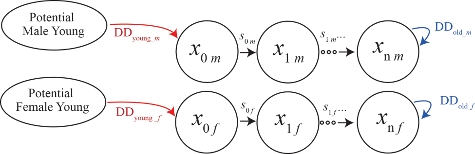
The following is a two-sex Leslie Matrix model expressed in terms of age-sex variables, time, life history survival, and natality parameters, where the female component of the model can be expressed as a matrix equation and the male component either requires doubling the dimension of the generalized Leslie matrix equation or augmenting the above equations with equations shown here.

Adjusted Leslie Matrix Equation

$$ \begin{eqnarray*} x_{1m}(t+1) & = & s_{0m} \sum_{i=1}^{n} b_{im}x_{if}(t) \nonumber \\ x_{i+1 \, m}(t+1) & = & s_{im} x_{im}(t) \ \ i=1,\dots, n-2 \\ x_{n \, m}(t+1) & = & s_{n-1 \, m} x_{n-1 \, m}(t) + s_{n m} x_{nm}(t) \nonumber \end{eqnarray*} $$

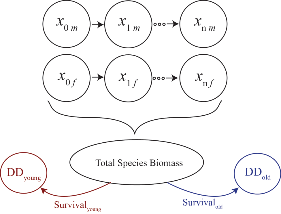
Density-Dependence Parameters

In terms of the aggregated population index:

$$ \begin{equation*} B_{i\ell}(t) = \sum_{j=1}^{n} \sum_{\ell = f,m} w_{ij\ell} x_{j\ell} (t), \end{equation*} $$

and corresponding case specific DD parameter, K, employs the DD-effects function:

$$ \begin{equation*} \phi = \frac{1}{1 + \left(\frac{B}{K} \right)^2} \end{equation*} $$

Stochasticity

$$ \begin{eqnarray*} x(t+1) = \mbox{BINOMIAL$[x(t),s]$} \end{eqnarray*} $$

$$ \begin{eqnarray*} x_{0,if}(t) & = & \mbox{BINOMIAL$[x_{0,i}(t),\rho_i]$} \end{eqnarray*} $$

$$ \begin{eqnarray*} x_{0,im}(t) & = & x_{0,i}(t) - x_{0,if}(t) \end{eqnarray*} $$

$$ \begin{eqnarray*} x_{1, i\ell}(t+1) & = & \sum_{i=1}^{n} F_{0,i \ell} s_{0,i\ell}x_{0, i\ell}(t) \ \ \ell=f,m \end{eqnarray*} $$

Demographic stochasticity arises in the context of survival of individuals when we regard survival parameters, s, as denoting probabilities that each individual survives rather than the proportion of individuals in the age class that survive. In this case, the variables are regarded as random variables that are determined from binomial distributions arising from repeated Bernoulli trials of whether or not each individual survives or does not survive with probabilities determined by s parameters.

Environmental stochasticity is easy to incorporate into the model in two different ways. First, in the functions the resources available to individuals in demographic class i can vary stochastically from one time period to the next. This is particularly easy to characterize if is treated purely as an input rather than a systems variable interacting with its consumers. Second, survival probabilities themselves can be treated as stochastic variables rather than constants. This can be done both in terms of large infrequent perturbations due to epidemics or other types of environmental catastrophes.

Conceptualizing Leslie Matrix

(Left) The total species biomass are calculated at each time step. Density dependence of young and old is calculated using both Total Species Biomass, an age-class specific weighted sum, and age-class specific survival rates.

(Below) A flow diagram of a two-sex, age-structured, population model with two sources of density-dependent survival in the youngest (DD young) and oldest (DD old) classes.

Transitions: Connectivity and Proclivity

meta-population dynamics respond in three steps: harvesting, stocking, and node-to-node transitions (in that order). All meta-population dynamics occur after standard demographic steps of the PVA. Transitions may occur between all unique subpopulations and the likelihood of transition is affected by both the age-class specific movement propensity of individuals and variable connectiity between meta-populations (displayed by the thickness of the arrows above). In addition, each unique meta-population has regional relative density dependence (DD values) for young that may or may not be used to motivate transitions.